ECLiPSeWiki | Examples / MipModels

Writing MIP models with ECLiPSe

First Example

This typical MIP model specification of a transport problem:

can be translated to ECLiPSe as follows:

    model(Capacities, Demands, Costs, Supply, Cost) :-

        dim(Costs, [M,N]),                              % get dimensions

        dim(Supply, [M,N]),                             % create variables
        Supply :: 0.0..inf,                             % ... with bounds

        ( for(J,1,M), param(Demands,Supply) do          % set up constraints
            sum(Supply[J,*]) $= Demands[J]
        ),

        ( for(I,1,N), param(Capacities,Supply) do
            sum(Supply[*,I]) $=< Capacities[I]
        ),

        Objective = sum(concat(Costs)*concat(Supply)),  % objective expression

        optimize(min(Objective), Cost).                 % solve

Parameters

Parameters are constants used in the model. They are either scalars or arrays of one or more dimensions. They can just be written as literals and assigned to ECLiPSe variables:

    NJobs = 10,

    Penalty = 3.5,

    Demand = [](43,12,65,0,5),

    C = [](
           [](  0,384,484,214),
	   [](384,  0,156,411),
	   [](484,156,  0,453),
	   [](214,411,453,  0)
          )

Larger data sets would usually be read from data files, which could be in various formats (ECLiPSe syntax, CSV, JSON, ...).

Variables

In MIP problems, variables are either continuous (reals) or integral (integers or binaries), and may have bounds: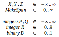

    reals([X,Y,Z]),              % continuous, no bounds
    MakeSpan $:: 0.0..inf,       % continuous, non-negative

    integers([P,Q]),             % integers, no bounds
    R $:: 0..9, integers([R]),   % integer between 0 and 9
    B $:: 0..1, integers([B]),   % binary

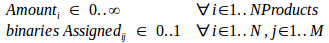Variables usually come in arrays of one or more dimensions. Create them with dim/2 and then give them their type and bound:

    dim(Amount, [NProducts]),    % array [1..NProducts]
    Amount $:: 0.0..inf          % continuous, non-negative

    dim(Assigned, [N,M]),        % 2D array [1..N,1..M]
    Assigned $:: 0..1,           % binaries
    integers(Assigned)