

The eplex library allows an external Mathematical Programming solver to be used by ECLiPSe. It is designed to allow the external solver to be seen as another solver for ECLiPSe, possibly in co-operation with the existing ‘native’ solvers of ECLiPSe such as the ic solver. It is not specific to a given external solver, with the differences between different solvers (largely) hidden from the user, so that the user can write the same code and it will run on the different solvers.
The exact types of problems that can be solved (and methods to solve them) are solver dependent, but currently linear programming, mixed integer programming and quadratic programming problems can be solved.
The rest of this chapter is organised as follows: the remainder of this introduction gives a very brief description of Mathematical Programming, which can be skipped if the reader is familiar with the concepts. Section 16.3 demonstrates the modelling of an MP problem, and the following section discusses some of the more advanced features of the library that are useful for hybrid techniques.
Mathematical Programming (MP) (also known as numerical optimisation) is the study of optimisation using mathematical/numerical techniques. A problem is modelled by a set of simultaneous equations: an objective function that is to be minimised or maximised, subject to a set of constraints on the problem variables, expressed as equalities and inequalities.
Many subclasses of MP problems have found important practical applications. In particular, Linear Programming (LP) problems and Mixed Integer Programming (MIP) problems are perhaps the most important. LP problems have both a linear objective function and linear constraints. MIP problems are LP problems where some or all of the variables are constrained to take on only integer values.
It is beyond the scope of this chapter to cover MP in any more detail. However, for most usages of the eplex library, the user need not know the details of MP – it can be treated as a black-box solver.
- Linear Programming (LP) problems: linear constraints and objective function, continuous variables.
- Mixed Integer Programming (MIP) problems: LP problems with some or all variables restricted to taking integral values.
Figure 16.1: Classification of MP problems
Much research effort has been devoted to developing efficient ways of solving the various subclasses of MP problems for over 50 years. The external solvers are state-of-the-art implementations of some of these techniques. The eplex library allows the user to model an MP problem in ECLiPSe, and then solve the problem using the best available MP tools.
In addition, the eplex library allows for the user to write programs that combines MP’s global algorithmic solving techniques with the local propagation techniques of Constraint Logic Programming.
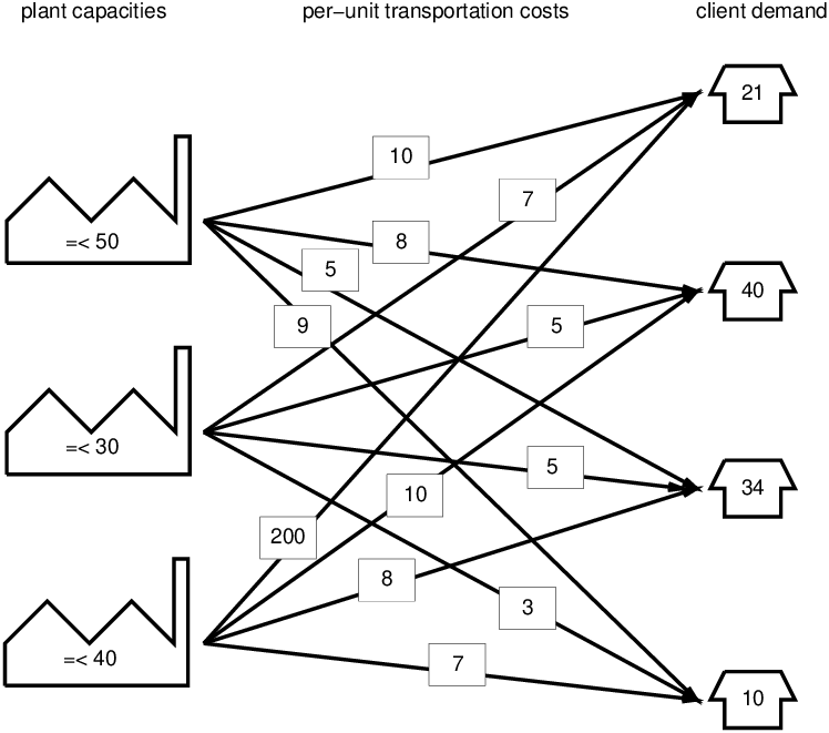
Figure 16.2: An Example MP Problem
Figure 16.2 shows an example of an MP problem. It is a transportation problem where several plants (1-3) have varying product producing capacities that must be transported to various clients (A-D), each requiring various amounts of the product. The per-unit cost of transporting the product to the clients also varies. The problem is to minimise the transportation cost whilst satisfying the demands of the clients.
To formulate the problem, we define the amount of product transported from a plant N to a client p as the variable Np, e.g. A1 represents the cost of transporting to plant A from client 1. There are two kinds of constraints:
The objective is to minimise the transportation cost, thus the objective function is to minimise the combined costs of transporting the product to all 4 clients from the 3 plants.
Putting everything together, we have the following formulation of the problem:
Objective function:
| min(10A1 + 7A2 + 200A3 + 8B1 + 5B2 + 10B3 + 5C1 + 5C2 + 8C3 + 9D1 + 3D2 + 7D3) |
Constraints:
|