Introduction

12.1 Introduction

In this chapter we will take a closer look at the principles and alternative methods of searching for solutions in the presence of constraints. Let us first recall what we are talking about. We assume we have the standard pattern of a constraint program:

solve(Data) :-
        model(Data, Variables),
        search(Variables),
        print_solution(Variables).

The model part contains the logical model of our problem. It defines the variables and the constraints. Every variable has a domain of values that it can take (in this context, we only consider domains with a finite number of values).

Once the model is set up, we go into the search phase. Search is necessary since generally the implementation of the constraints is not complete, i.e. not strong enough to logically infer directly the solution to the problem. Also, there may be multiple solutions which have to be located by search, e.g. in order to find the best one. In the following, we will use the following terminology:

If a variable is given a value (from its domain, of course), we call this an assignment. If every problem variable is given a value, we call this a total assignment.
A total assignment is a solution if it satisfies all the constraints.
The search space is the set of all possible total assignments. The search space is usually very large because it grows exponentially with the problem size:
SearchSpaceSize = DomainSize^{NumberOfVariables}

12.1.1 Overview of Search Methods

Figure 12.1: A search space of size 16

Figure 12.1 shows a search space with N (here 16) possible total assignments, some of which are solutions. Search methods now differ in the way in which these assignments are visited. We can classify search methods according to different criteria:

Complete vs incomplete exploration: complete search means that the search space is investigated in such a way that all solutions are guaranteed to be found. This is necessary when the optimal solution is needed (one has to prove that no better solution exists). Incomplete search may be sufficient when just some solution or a relatively good solution is needed.
Constructive vs move-based: this indicates whether the method advances by incrementally constructing assignments (thereby reasoning about partial assignments which represent subsets of the search space) or by moving between total assignments (usually by modifying previously explored assignments).
Randomness: some methods have a random element while others follow fixed rules.

Here is a selection of search methods together with their properties:

Method	exploration	assignments	random
Full tree search	complete	constructive	no
Credit search	incomplete	constructive	no
Bounded backtrack	incomplete	constructive	no
Limited discrepancy	complete	constructive	no
Hill climbing	incomplete	move-based	possibly
Simulated annealing	incomplete	move-based	yes
Tabu search	incomplete	move-based	possibly
Weak commitment	complete	hybrid	no

The constructive search methods usually organise the search space by partitioning it systematically. This can be done naturally with a search tree (Figure 12.2). The nodes in this tree represent choices which partition the remaining search space into two or more (usually disjoint) sub-spaces. Using such a tree structure, the search space can be traversed systematically and completely (with as little as O(N) memory requirements).

Figure 12.2: Search space structured using a search tree

Figure 12.4 shows a sample tree search, namely a depth-first incomplete traversal. As opposed to that, figure 12.3 shows an example of an incomplete move-based search which does not follow a fixed search space structure. Of course, it will have to take other precautions to avoid looping and ensure termination.

Figure 12.3: A move-based search

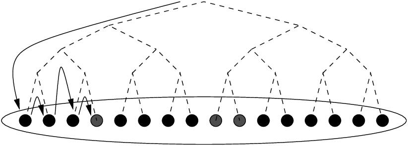
Figure 12.4: A tree search (depth-first)

A few further observations: Move-based methods are usually incomplete. This is not surprising given typical sizes of search spaces. A complete exploration of a huge search space is only possible if large sub-spaces can be excluded a priori, and this is only possible with constructive methods which allow one to reason about whole classes of similar assignments. Moreover, a complete search method must remember which parts of the search space have already been visited. This can only be implemented with acceptable memory requirements if there is a simple structuring of the space that allows compact encoding of sub-spaces.

12.1.2 Optimisation and Search

Many practical problems are in fact optimisation problems, ie. we are not just interested in some solution or all solutions, but in the best solution.

Fortunately, there is a general method to find the optimal solution based on the ability to find all solutions. The branch-and-bound technique works as follows:

Find a first solution
Add a constraint requiring a better solution than the best one we have so far (e.g. require lower cost)
Find a solution which satisfies this new constraint. If one exists, we have a new best solution and we repeat step 2. If not, the last solution found is the proven optimum.

The branch_and_bound library provides generic predicates which implement this technique:

minimize(+Goal,-Cost): This is the simplest predicate in the branch_and_bound library: A solution of the goal Goal is found that minimizes the value of Cost. Cost should be a variable that is affected, and eventually instantiated, by the execution of Goal. Usually, Goal is the search procedure of a constraint problem and Cost is the variable representing the cost.
bb_min(+Goal, -Cost, ++Options): A more flexible version where the programmer can take more control over the branch and bound behaviour and choose between different strategies and parameter settings.

12.1.3 Heuristics

Since search space sizes grow exponentially with problem size, it is not possible to explore all assignments except for the very smallest problems. The only way out is not to look at the whole search space. There are only two ways to do this:

Prove that certain areas of the space contain no solutions. This can be done with the help of constraints. This is often referred to as pruning.
Ignore parts of the search space that are unlikely to contain solutions (i.e. do incomplete search), or at least postpone their exploration. This is done by using heuristics. A heuristic is a particular traversal order of the search space which explores promising areas first.

In the following sections we will first investigate the considerable degrees of freedom that are available for heuristics within the framework of systematic tree search, which is the traditional search method in the Constraint Logic Programming world.

Subsequently, we will turn our attention to move-based methods which in ECLⁱPS^e can be implemented using the facilities of the repair library.