


In very simple cases, just imposing the constraints may be sufficient to directly compute the (unique) solution. For example:
?- 3 * X $= 4.
X = 1.3333333333333333__1.3333333333333335
Yes
Other times, propagation will reduce the domains of the variables to suitably small intervals:
?- 3 * X + 2 * Y $= 4, X - 5 * Y $= 2, X $>= -100.
Y = Y{-0.11764705946382902 .. -0.1176470540212896}
X = X{1.4117647026808551 .. 1.4117647063092196}
There are 2 delayed goals.
Yes
In general though, some extra work will be needed to find the solutions of a problem. The IC library provides two methods for assisting with this. Which method is appropriate depends on the nature of the solutions to be found. If it is expected that there a finite number of discrete solutions, locate/2 and locate/3 would be good choices. If solutions are expected to lie in a continuous region, squash/3 may be more appropriate.
Locate works by nondeterministically splitting the domains of the variables until they are narrower than a specified precision (in either absolute or relative terms). Consider the problem of finding the points where two circles intersect (see Figure 9.4). Normal propagation does not deduce more than the obvious bounds on the variables:

Figure 9.4: Example of using locate/2
?- 4 $= X^2 + Y^2, 4 $= (X - 1)^2 + (Y - 1)^2.
X = X{-1.0000000000000004 .. 2.0000000000000004}
Y = Y{-1.0000000000000004 .. 2.0000000000000004}
There are 12 delayed goals.
Yes
Calling locate/2 quickly determines that there are two solutions and finds them to the desired accuracy:
?- 4 $= X^2 + Y^2, 4 $= (X-1)^2 + (Y-1)^2, locate([X, Y], 1e-5).
X = X{-0.8228756603552696 .. -0.82287564484820042}
Y = Y{1.8228756448482002 .. 1.8228756603552694}
There are 12 delayed goals.
More

X = X{1.8228756448482004 .. 1.8228756603552696}
Y = Y{-0.82287566035526938 .. -0.82287564484820019}
There are 12 delayed goals.
Yes
Squash works by deterministically cutting off parts of the domains of variables which it determines cannot contain any solutions. In effect, it is like a stronger version of bounds propagation. Consider the problem of finding the intersection of two circular discs and a hyperplane (see Figure 9.5). Again, normal propagation does not deduce more than the obvious bounds on the variables:
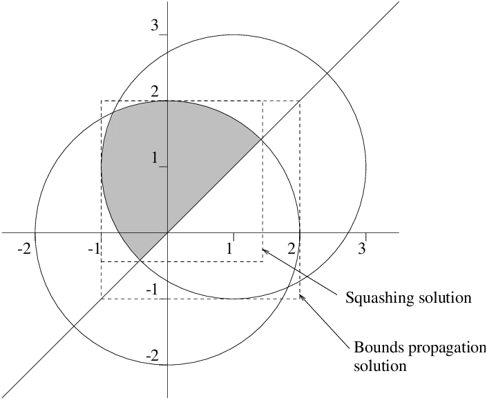
Figure 9.5: Example of propagation using the squash algorithm
?- 4 $>= X^2 + Y^2, 4 $>= (X-1)^2 + (Y-1)^2, Y $>= X.
Y = Y{-1.0000000000000004 .. 2.0000000000000004}
X = X{-1.0000000000000004 .. 2.0000000000000004}
There are 13 delayed goals.
Yes
Calling squash/3 results in the bounds being tightened (in this case the bounds are tight for the feasible region, though this is not true in general):
?- 4 $>= X^2 + Y^2, 4 $>= (X-1)^2 + (Y-1)^2, Y $>= X,
   squash([X, Y], 1e-5, lin).
X = X{-1.0000000000000004 .. 1.4142135999632601}
Y = Y{-0.41421359996326 .. 2.0000000000000004}
There are 13 delayed goals.
Yes