• View
• Edit
• History
• Print

SquareSumChain

Solving the Square-Sum-Chain problem

Author: Joachim Schimpf, February 2018, under Creative Commons Attribution-ShareAlike 4.0 International License

The Challenge

The problem is easy to describe:

For example:

    8 1 15 10 6 3 13 12 4 5 11 14 2 7 9

where 8+1 = 3^2, 1+15 = 4^2, 10+6 = 4^2, 6+3 = 3^2, etc. The smallest N for which a solution exists is 15; no solutions exist for 18,19,20,21,22 and 24. Beyond that, solutions seem to always exist, but to our knowledge there is no proof.

The problem is explained and further discussed in the following places

• Numberphile Youtube video
• Reddit programming challenge
• Stackoverflow topic

In the following, we develop a number of alternative solutions in ECLiPSe (some require at least version 7.0). All programs are short, 10-20 lines of code.

1. Prolog-style backtrack search
2. Constrained search - alldifferent and arithmetic constraints
3. Constrained search - table constraint
4. Constrained search - circuit constraint
5. Comparison of constraint-based solutions
6. Algorithmic methods
7. Visualization

Executive Summary

One of the constraint-based solutions performs best and scales up to thousands of elements.

Prolog-style backtrack search

The following is a straightforward Prolog backtracking solution, except that we use ECLiPSe's do-loop construct to avoid the need for auxiliary clauses:

    ssc_prolog(N, Xs) :-
        ( for(I,1,N), foreach(I,Ns) do true ),     % construct a list Ns = [1,...,N]
        select(X1, Ns, Ns1),                       % pick a first number X1
        (                                          % Iterate over:
            fromto(X1,X2,X3,XN),                   % - first element of a pair
            fromto(Ns1,Ns2,Ns3,[]),                % - remaining numbers
            fromto(Xs,[X2|Xs3],Xs3,[XN])           % - the result list
        do
            select(X3, Ns2, Ns3),                  % pick a next number X3
            square_sum(X2, X3)
        ).

    square_sum(X, Y) :-                            % check if (X,Y) is a valid pair
        R is sqrt(X+Y),
        R =:= round(R)

Here, nondeterministic choices are made by lists:select/3, and the pair condition is tested using standard functional arithmetic.

This solves small instances easily:

    ?- ssc_prolog(15, Xs).
    Xs = [8, 1, 15, 10, 6, 3, 13, 12, 4, 5, 11, 14, 2, 7, 9]
    Yes (0.00s cpu, solution 1, maybe more)
    Xs = [9, 7, 2, 14, 11, 5, 4, 12, 13, 3, 6, 10, 15, 1, 8]
    Yes (0.00s cpu, solution 2, maybe more)
    No (0.00s cpu)

However, solving times start to increase quickly, and N=50 already takes over a minute.

Constrained search - alldifferent and arithmetic constraints

Next, we try a formulation with constraints, using the library(ic) constraint solver.

We simply create an array of integer variables ranging from 1 to N. We state that all the numbers must be different, and then (in a loop) we constrain the sum of each consecutive pair to be equal to the square of some positive integer R:

    :- lib(ic).

    ssc_arith(N, Xs) :-
        dim(Xs, [N]),                          % array of integer variables 1..N
        Xs #:: 1..N,
        ic_global:alldifferent(Xs),            % all numbers must be different
        ( for(I,1,N-1), param(Xs) do           % iterate over pairs Xs[I],Xs[I+1]
	    R #> 0,
            Xs[I] + Xs[I+1] #= sqr(R)         % sum is square of some integer R
        ),
        search(Xs, 0, input_order, indomain_max, complete, []).

Finally, we invoke the built-in search routine search/6. The search options we have chosen are the most naive ones, except that we use indomain_max instead of indomain/indomain_min: this has the effect of trying larger domain values first. As the first two columns of the comparison table show, this is advantageous in most cases.

Constrained search - table constraint

One reason for the previous model to perform badly is that we used the arithmetic constraint X[I]+X[I+1] #= sqr(R) to restrict the values of X[I],X[I+1] pair. This constraint does not propagate very strongly.

Another way to model this is with a table/2 constraint: we can precompute a table of all valid pairs of values (i.e. pairs of values between 1 and N that add up to a square), and enforce the constraint that every variable pair must take their values from the table.

The following code first solves the 2-variable subproblem in sum_is_square/2 and computes a table of all solutions, using findall/3. This table [[1,3],[1,8],[1,15],...] is then used to set up the table/2 constraint on all the consecutive variable pairs in the full problem.

    ssc_table(N, Xs) :-
        dim(Xs, [N]),
        Xs #:: 1..N,
        ic_global:alldifferent(Xs),
        sum_is_square(N, Table),
        ( for(I,1,N-1), foreach([X,Y],Pairs), param(Xs) do
            subscript(Xs, [I], X),
            subscript(Xs, [I+1], Y)
        ),
        ic_global_gac:table(Pairs, Table),
        search(Xs, 0, input_order, indomain_max, complete, []).

    sum_is_square(N, Table) :-
        findall([X,Y], (
            [X,Y,R] #:: 1..N,
            X #\= Y,
            X + Y #= sqr(R),
            labeling([X,Y,R])
        ), Table).

Compared to the previous model, this improves things by about an order of magnitude, but we still get timeouts below problem size 50!

We can try to exploit the same idea in a stronger way: instead of precomputing a 2-variable sub-problem, we can precompute all solutions to a 3-variable subproblem: [[1,3,6],[1,3,13],...]. This can be used to impose table-constraints on every consective triplet of variables in the full problem:

    ssc_table3(N, Xs) :-
        dim(Xs, [N]),
        Xs #:: 1..N,
        ic_global:alldifferent(Xs),
        sum_is_square3(N, Table),
        ( for(I,1,N-2), foreach([X,Y,Z],Triplets), param(Xs) do
            subscript(Xs, [I], X),
            subscript(Xs, [I+1], Y),
            subscript(Xs, [I+2], Z)
        ),
        ic_global_gac:table(Triplets, Table),
        search(Xs, 0, input_order, indomain_max, complete, [])

    sum_is_square3(N, Table) :-
        findall([X,Y,Z], (
            [X,Y,Z,R1,R2] #:: 1..N,
            alldifferent([X,Y,Z]),
            X + Y #= sqr(R1),
            Y + Z #= sqr(R2),
            labeling([X,Y,Z,R1,R2])
        ), Table).

We have now (N-2) 3-variable-constraints, each of which overlaps in two variables with the previous constraint. Note that this is redundant: it would be enough to have the constraints overlapping in only one variable. However, the larger overlap allows stronger propagation. As the results show, the gains are significant.

Unfortunately, for larger N this method becomes impractical again, because the 3-variable subproblems start having too many solutions, taking long to compute and leading to very large tables.

Constrained search - circuit constraint

This model takes advantage of the circuit/1 constraint, which enforces Hamiltonian circuits (and can be used to enforce a Hamiltonian path by adding a dummy source/sink node to close the circuit). The constraint works on a graph represented as a successor array: S[I]=J means that there is an edge from I to J.

We compute the initial successor domain for a node I by taking all integers that form a valid square-sum pair with I. Then we add a starting node and set up the circuit-constraint:

    ssc_circuit(N, Xs) :-
        N1 is N+1,                    % add source/sink node Sz[N+1]
        dim(Sz, [N1]),                % array of successor variables
        ( for(I,1,N), param(Sz,N) do
            arg(I, Sz, J),            % J is the successor node of I
                                      % find all K compatible with I
            findall(K, (between(1,N,1,K), square_sum(I,K) ; K is N+1), Ks),
            J #:: Ks                  % J can take all values compatible with I
        ),
        Sz[N1] #:: 1..N,              % starting node
        circuit(Sz),
        search(Sz, 0, first_fail, indomain_max, lds(1), []),

        % map successor array to node list path, for output
        arg(N1, Sz, X0),
        ( fromto(X0,X,X1,N1), foreach(X,Xs), param(Sz) do
            arg(X, Sz, X1)
        ).

After a solution has been found, the successor array is translated to a node list, giving the resulting path in a more readable form.

This model performs well (even with the naive input_order variable selection strategy), encountering its first timeout at N=236.

Switching to a better variable selection strategy (first_fail) improves things further, but there are still outliers for difficult instances, where the search gets stuck in parts of the search tree.

To overcome this issue, as a last improvement we switch from naive complete depth-first search to Least Discrepancy Search (lds(1)). The last results column shows that this consistently solves even larger instances (thousands) efficiently.

Comparison of constraint-based solutions

We used a time-out of 60 seconds, and the numbers listed give the number of backtracks necessary to find a first solution.

The number of backtracks can be obtained by giving the backtrack(BT) option to the search/6 procedure, e.g.

    ...
    search(Xs, 0, input_order, indomain_max, complete, [backtrack(BT)]),
    writeln(number_of_backtracks(BT)).

Algorithmic methods - explicit graph search

Most of the solutions in imperative programming languages (such as those in [1]) use an explicit algorithm to create a graph of compatible numbers, and then perform a search for a Hamiltonian path in the graph.

We can do this as well: We first compute a graph representation in the form of an array of node-stuctures node(X,Ys,Step), where X is the node number and Ys is a list of node numbers Y, such that (X,Y) is a valid square-sum pair. The third component, Step is initially uninstantiated.

The second phase is depth-first search, exploiting Prolog's nondeterminism: we nondeterministically pick a starting node, and then nondeterministically pick outgoing edges from each node reached. Subtours are excluded by marking each node with its position in the path (Step):

    ssc_graph_simple(N, Xs) :-
        dim(G, [N]),                        % graph is an array of nodes
        ( foreacharg(node(X,Ys,_),G,X), param(N) do
            findall(Y, (between(1,N,1,Y), X\=Y, square_sum(X,Y)), Ys)
        ),
        between(1, N, 1, Start),            % pick starting node
        (
            for(Step,1,N),
            foreach(X,Xs),
            fromto(Start,X,Y,_End),
            param(G)
        do
            arg(X, G, node(X,Ys,Step)),
            member(Y,Ys)                    % pick successor
        ).

This works reasonably well up to N=55, but then quickly starts timing out.

We can improve upon the algorithm by incorporating heuristics, such as picking nodes with few outgoing edges first (this corresponds to the first_fail heuristic in constrained search). This involves some additional data structures, sorting, etc:

    ssc_graph(N, Xs) :-
        % Build graph of node(Nr,OutDegree,Successors,OrderedSuccessors,PathPosition)
        dim(G, [N]),
        ( foreacharg(node(X,Degree,Ys,_,_),G,X), param(N) do
            findall(Y, (between(1,N,1,Y), X\=Y, square_sum(X,Y)), Ys),
            length(Ys, Degree)
        ),
        % order all successor lists by increasing Degree
        ( foreacharg(node(_X,_Degree,Ys,SYs,_),G), param(G) do
            sort_nodes_by_degree(Ys, G, SYs)
        ),
        % make a start node list, also ordered by OutDegree
        ( for(I,1,N), foreach(I,Is) do true ),
        sort_nodes_by_degree(Is, G, Starts),
        % find path
        (
            for(Step,1,N),
            fromto(Starts,Ss,Ys,_),
            foreach(X,Xs),
            param(G)
        do
            member(X, Ss),
            arg(X, G, node(X,_Degree,_Ys,Ys,Step))
        ).

    sort_nodes_by_degree(Is, G, SIs) :-
        ( foreach(I,Is), foreach(Node,Nodes), param(G) do arg(I, G, Node) ),
        sort(2, =<, Nodes, SortedNodes),
        ( foreach(node(I,_,_,_,_),SortedNodes), foreach(I,SIs) do true ).

Despite the extra effort and some improvement, this still does not scale well beyond about N=80, leaving the best constraint-based solutions as the method of choice.

Visualizing the problem

To see the pair compatibility graph, use ECLiPSe's graph tools:

    :- lib(graph_algorithms).
    :- lib(graphviz).

    ssc_view_graph(N) :-
        findall(e(X,Y,1), (
            between(1, N, 1, X),
            between(1, N, 1, Y),
            X\=Y,
            square_sum(X,Y)
        ), Edges),
        make_graph(N, Edges, G),
        view_graph(G, [layout:left_to_right]).

The output of ssc_view_graph(15) is: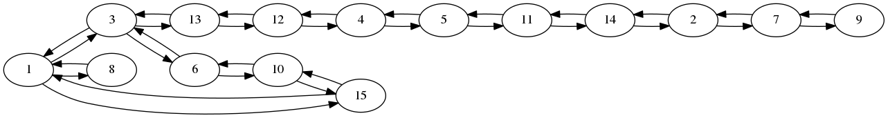