


Part of the power of using the eplex library comes from being able to solve
an eplex problem repeatedly after modification.
For example, we can solve the original transportation
problem, add the extra constraint, and resolve the problem.
Remember that as eplex_solve/1 instantiates its argument, we
need to use a new variable for each call:
|
Note that posted constraints behave logically: they are added to an eplex instance when posted, and removed when they are backtracked over.
In the examples so far, the solver has been invoked explicitly. However, the solver can also behave like a normal constraint, i.e. it is automatically invoked when certain conditions are met.
As an example, we implement the standard branch-and-bound method of solving a MIP problem, using the external solver as an LP solver only. Firstly we outline how this can be implemented with the facilities we have already encountered. We then show how this can be improved usin more advanced features of lib(eplex).
With the branch-and-bound approach, a search-tree is formed, and at each node a ‘relaxed’ version of the MIP problem is solved as an LP problem. Starting at the root, the problem solved is the original MIP problem, but without any of the integrality constraints:
|
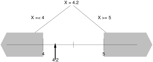
Figure 16.5: Labelling a variable at a MIP tree node
In general, this initial LP solution contains non-integer assignments to integer variables. The objective value of this LP is a lower bound on the actual MIP objective value. The task of the search is to find integer assignments for the integer variables that optimises the objective function. Each node of the search-tree solves the problem with extra bound constraints on these variables. At each node, a particular variable is ‘labelled’ as shown in Figure 16.5. The integer variable in this case has been assigned the non-integer value of 4.2. In the subsequent nodes of the tree, we consider two alternate problems, which creates two branches in the search. In one problem, we impose the bound constraint X ≤ 4, and in the other, X ≥ 5: these are the two nearest integer values to 4.2. In each branch, the problem is solved again as an LP problem with its new bound for the variable:
|
A choice-point for the two alternative branchings is created in the above
code, the problem is solved with one of the branchings (X $=< Split).
The program then proceeds to further labelling of the variables. The
alternative branch is left to be tried on backtracking.
Eventually, if the problem has a solution, all the integer variables will be ‘labelled’ with integer values, resulting in a solution to the MIP problem. However, this will generally not be optimal, and so the program needs to backtrack into the tree to search for a better solution by trying the other branches for the variables, using the existing solution value as a bound. This ‘branch-and-bound’ search technique is implemented in lib(branch_and_bound).
Remember that ECLiPSe provides libraries that make some programming tasks much easier. There is no need to write your own code when you can use what is provided by an ECLiPSe library.
Figure 16.6: Reminder: use ECLiPSe libraries!
In the code, the external solver is invoked explicitly at every node. This
however may not be necessary as the imposed bound may already be satisfied.
As stated at the start of this section, the invocation of the solver could be done in a
data-driven way, more like a normal constraint.
This is done with eplex_solver_setup/4:
eplex_solver_setup(+Obj,-ObjVal,+Options,+Trigs), a more
powerful version of eplex_solver_setup/1 for setting up a
solver. The Trigs argument specifies a list of ‘trigger
modes’ for triggering the solver.
For our example, we add a bound constraint at each node to exclude a
fractional solution value for a variable. The criterion we want to use is
to invoke the solver only if this old solution value is excluded by the new
bounds (otherwise the external solver will solve the same problem
redundantly). This is done by
specifying deviating_bounds in the trigger modes.
The full code that
implements a MIP solution for the
example transportation problem is given below:
|
The setup of the solver is done in line k, with the use of the
deviating_bounds trigger mode. There are no explicit calls to trigger the
solver – it is triggered automatically. In addition, the first call to
eplex_solve/1 for an initial solution
is also not required, because when trigger modes are specified, then
by default, eplex_solver_setup/4 will invoke the solver once the
problem is setup.
Besides the deviating_bounds
trigger condition, the other argument of interest in our use of
eplex_solver_setup/4 is the second argument,
the objective value of the problem (Cost in the example):
recall that this was returned previously by eplex_solve/1.
Unlike in eplex_solve/1, the variable is not
instantiated when the solver returns. Instead, one of the bounds (lower
bound in the case of minimise) is updated
to the optimal value, reflecting the range the objective value can take,
from suboptimal to the ‘best’ value at optimal. The variable is therefore
made a problem variable by posting of the objective as a constraint in line
j. This informs the external solver needs to be informed
that the Cost variable is the objective value.
In line m, the branch choice is created by the posting of the bound
constraint, which may trigger the external solver. Here, we use a
simple heuristic to decide which of the two branches to try first: the
branch with the integer range closer to the relaxed solution value.
For example, in the situation of Figure 16.5, the branch with
X $=< 4 is tried first since the solution value of 4.2 is
closer to 4 than 5.
By using lib(branch_and_bound)’s bb_min/3 predicate in m,
there is no need to explicitly write our own branch-and-bound routine. However,
this predicate requires the cost variable to be instantiated, so we call
eplex_get(cost, Cost) to instantiate Cost at the end of
each labelling of the variables. We also get the solution values for the
variables, so that the branch-and-bound routine will remember it.
The final value returned in Cost (and Vars for the solution
values)
is the optimal value after the branch-and-bound search, i.e. the
optimal value for the MIP problem.
- Use Instance:eplex_solver_setup(+Obj,-ObjVal,+Opts,+Trigs) to set up an external solver state for instance Instance. Trigs specifies a list of trigger conditions to automatically trigger the external solver.
- Instance:eplex_var_get(+Var,+What,-Value) can be used to obtain information for the variable Var in the eplex instance.
- Instance:eplex_get(+Item, -Value) can be used to retrieve information about the eplex instance’s solver state.
Figure 16.7: More advanced modelling in eplex
Of course, in practice, we do not write our own MIP solver, but use the MIP solver provided with the external solvers instead. These solvers are highly optimised and tightly coupled to their own LP solvers. The techniques of solving relaxed subproblems described here are however very useful for combining the external solver with other solvers in a hybrid fashion.